import matplotlib.pyplot as plt
import numpy as np
import sympy as sy

sy.init_printing()
Consider two vectors \(u\) and \(v\) in \(\mathbb{R}^2\), they are independent of each other, i.e. not pointing to the same or opposite direction. Therefore any vector in the \(\mathbb{R}^2\) can be represented by a linear combination of \(u\) and \(v\).
For instance, this is a linear combination and essentially a linear system.
\[ c_1 \left[ \begin{matrix} 4\\ 2 \end{matrix} \right]+ c_2 \left[ \begin{matrix} -2\\ 2 \end{matrix} \right] = \left[ \begin{matrix} 2\\ 10 \end{matrix} \right] \]
Solve the system in SymPy:
A = sy.Matrix([[4, -2, 2], [2, 2, 10]])
A.rref()
\(\displaystyle \left( \left[\begin{matrix}1 & 0 & 2\\0 & 1 & 3\end{matrix}\right], \ \left( 0, \ 1\right)\right)\)
The solution is \((c_1, c_2)^T = (2, 3)^T\), which means the addition of \(2\) times \(\left[ \begin{matrix} 4\\ 2 \end{matrix} \right]\) and \(3\) times \(\left[ \begin{matrix} -2\\ 2 \end{matrix} \right]\) equals \(\left[ \begin{matrix} 2\\ 10 \end{matrix} \right]\).
Besides plotting the vector addition, we would like to plot the coordinates of the basis spanned by \(u\) and \(v\). We will explain this further in a later chapter.
Calculate the slope of the vectors, i.e., \(\frac{y}{x}\): \[ s_1 = \frac{y}{x} = \frac{2}{4} = 0.5 \\ s_2 = \frac{y}{x} = \frac{2}{-2} = -1 \]
The basis can be constructed as: \[ y_1 = a + 0.5x \\ y_2 = b - x \] where \(a\) and \(b\) will be set as constants with regular intervals, such as \((2.5, 5, 7.5, 10)\).
The coordinates of the basis are represented as pink web-style grids, where each line segment is a unit (like \(1\) in the Cartesian coordinate system) in the ‘new’ coordinates.
# Initialize the figure and axis
fig, ax = plt.subplots(figsize=(8, 8))

# Define the vectors and their colors
vectors = np.array(
    [[[0, 0, 4, 2]], [[0, 0, -2, 2]], [[0, 0, 2, 10]], [[0, 0, 8, 4]], [[0, 0, -6, 6]]]
)
colors = ["b", "b", "r", "b", "b"]

# Plot each vector with quiver and add annotations
for i in range(vectors.shape[0]):
    X, Y, U, V = zip(*vectors[i, :, :])
    ax.quiver(
        X, Y, U, V, angles="xy", scale_units="xy", color=colors[i], scale=1, alpha=0.6
    )
    ax.text(
        x=vectors[i, 0, 2],
        y=vectors[i, 0, 3],
        s="$(%.0d, %.0d)$" % (vectors[i, 0, 2], vectors[i, 0, 3]),
        fontsize=16,
    )

# Highlight the linear combination lines
points12 = np.array([[8, 4], [2, 10]])
ax.plot(points12[:, 0], points12[:, 1], color="b", lw=3.5, alpha=0.5, ls="--")

points34 = np.array([[-6, 6], [2, 10]])
ax.plot(points34[:, 0], points34[:, 1], color="b", lw=3.5, alpha=0.5, ls="--")

# Set axis limits and labels
ax.set_xlim([-10, 10])
ax.set_ylim([0, 10.5])
ax.set_xlabel("x-axis", fontsize=16)
ax.set_ylabel("y-axis", fontsize=16)
ax.grid()

# Plot the basis lines
a = np.arange(-11, 20, 1)
x = np.arange(-11, 20, 1)

for i in a:
    y1 = i + 0.5 * x
    ax.plot(x, y1, ls="--", color="pink", lw=2)
    y2 = i - x
    ax.plot(x, y2, ls="--", color="pink", lw=2)

# Add title using a raw string
ax.set_title(
    r"Linear Combination of Two Vectors in $\mathbf{R}^2$", size=22, x=0.5, y=1.01
)

# Show the plot
plt.show()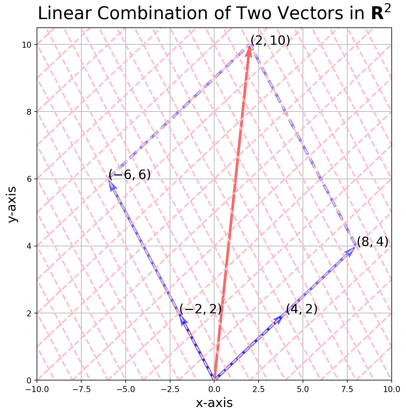
Linear Combination Visualization in 3D
We can also show that any vectors in \(\mathbb{R}^3\) can be a linear combination of a standard basis in Cartesian coordinate system.
Here is the function for plotting 3D linear combination from standard basis, we just feed the scalar multiplier.
def linearCombo(a, b, c):
    """This function is for visualizing linear combination of standard basis in 3D.
    Function syntax: linearCombo(a, b, c), where a, b, c are the scalar multiplier,
    also the elements of the vector.
    """
    fig = plt.figure(figsize=(10, 10))
    ax = fig.add_subplot(111, projection="3d")
    ######################## Standard basis and Scalar Multiplid Vectors#########################
    vec = np.array(
        [
            [[0, 0, 0, 1, 0, 0]],  # e1
            [[0, 0, 0, 0, 1, 0]],  # e2
            [[0, 0, 0, 0, 0, 1]],  # e3
            [[0, 0, 0, a, 0, 0]],  # a* e1
            [[0, 0, 0, 0, b, 0]],  # b* e2
            [[0, 0, 0, 0, 0, c]],  # c* e3
            [[0, 0, 0, a, b, c]],
        ]
    )  # ae1 + be2 + ce3
    colors = ["b", "b", "b", "r", "r", "r", "g"]
    for i in range(vec.shape[0]):
        X, Y, Z, U, V, W = zip(*vec[i, :, :])
        ax.quiver(
            X,
            Y,
            Z,
            U,
            V,
            W,
            length=1,
            normalize=False,
            color=colors[i],
            arrow_length_ratio=0.08,
            pivot="tail",
            linestyles="solid",
            linewidths=3,
            alpha=0.6,
        )

    #################################Plot Rectangle Boxes##############################
    dlines = np.array(
        [
            [[a, 0, 0], [a, b, 0]],
            [[0, b, 0], [a, b, 0]],
            [[0, 0, c], [a, b, c]],
            [[0, 0, c], [a, 0, c]],
            [[a, 0, c], [a, b, c]],
            [[0, 0, c], [0, b, c]],
            [[0, b, c], [a, b, c]],
            [[a, 0, 0], [a, 0, c]],
            [[0, b, 0], [0, b, c]],
            [[a, b, 0], [a, b, c]],
        ]
    )
    colors = ["k", "k", "g", "k", "k", "k", "k", "k", "k"]
    for i in range(dlines.shape[0]):
        ax.plot(
            dlines[i, :, 0],
            dlines[i, :, 1],
            dlines[i, :, 2],
            lw=3,
            ls="--",
            color="black",
            alpha=0.5,
        )

    #################################Annotation########################################
    ax.text(x=a, y=b, z=c, s=" $(%0.d, %0.d, %.0d)$" % (a, b, c), size=18)
    ax.text(x=a, y=0, z=0, s=" $%0.d e_1 = (%0.d, 0, 0)$" % (a, a), size=15)
    ax.text(x=0, y=b, z=0, s=" $%0.d e_2 = (0, %0.d, 0)$" % (b, b), size=15)
    ax.text(x=0, y=0, z=c, s=" $%0.d e_3 = (0, 0, %0.d)$" % (c, c), size=15)

    #################################Axis Setting######################################
    ax.grid()
    ax.set_xlim([0, a + 1])
    ax.set_ylim([0, b + 1])
    ax.set_zlim([0, c + 1])

    ax.set_xlabel("x-axis", size=18)
    ax.set_ylabel("y-axis", size=18)
    ax.set_zlabel("z-axis", size=18)

    ax.set_title("Vector $(%0.d, %0.d, %.0d)$ Visualization" % (a, b, c), size=20)

    ax.view_init(elev=20.0, azim=15)


if __name__ == "__main__":
    a = 7
    b = 4
    c = 9
    linearCombo(a, b, c)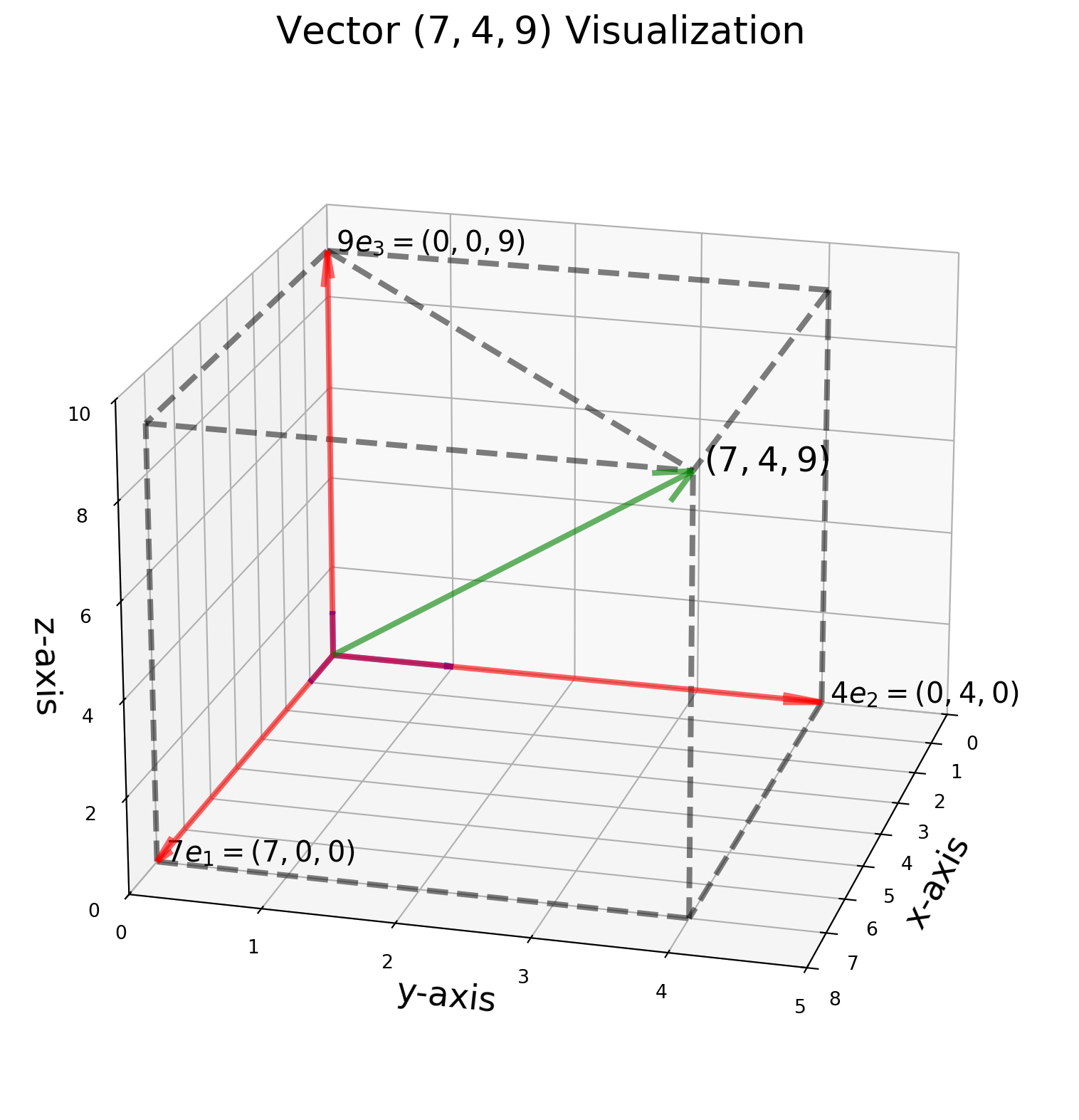
linearCombo(3, 5, 6) # Try again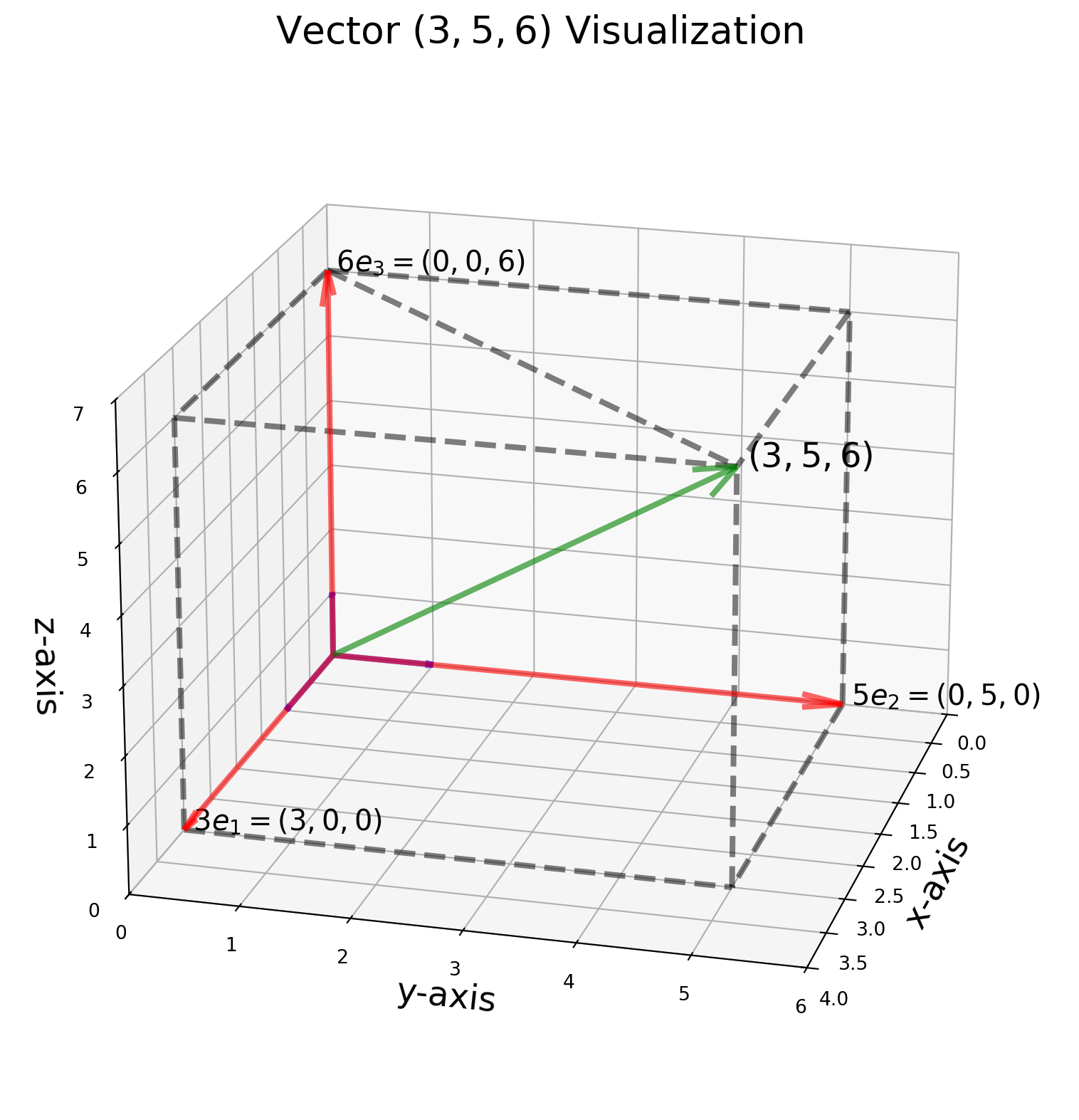
Linear Combination of Inconsistent System
An inconsistent system means no unique solution exists. It might seem strange to treat a solution of an inconsistent system as a linear combination, but it essentially represents a trace of a line.
One Free Variable Case
We have seen how inconsistent systems can be solved in the earlier lectures. Now we will investigate what solution means from the perspective of linear combination.
Consider a system
\[ \left[ \begin{matrix} 1 & 1 & 2\\ -2 &0 & 1\\ 1& 1 & 2 \end{matrix} \right] \left[ \begin{matrix} c_1\\c_2\\c_3 \end{matrix} \right] = \left[ \begin{matrix} 1\\-3\\1 \end{matrix} \right] \]
Solve in SymPy:
A = sy.Matrix([[1, 1, 2, 1], [-2, 0, 1, -3], [1, 1, 2, 1]])
A.rref()
\(\displaystyle \left( \left[\begin{matrix}1 & 0 & - \frac{1}{2} & \frac{3}{2}\\0 & 1 & \frac{5}{2} & - \frac{1}{2}\\0 & 0 & 0 & 0\end{matrix}\right], \ \left( 0, \ 1\right)\right)\)
The solution is not unique due to a free variable:
\[ c_1 - \frac{1}{2}c_3 =\frac{3}{2}\\ c_2 + \frac{5}{2}c_3 = -\frac{1}{2}\\ c_3 = free \]
Let \(c_3 = t\), the system can be parameterized:
\[ \left[ \begin{matrix} c_1\\c_2\\c_3 \end{matrix} \right] = \left[ \begin{matrix} \frac{3}{2}+\frac{1}{2}t\\ -\frac{1}{2}-\frac{5}{2}t\\ t \end{matrix} \right] \]
The solution is a line of infinite length, to visualize it, we set the range of \(t\in (-1, 1)\), the solution looks like:
fig = plt.figure(figsize=(8, 8))
ax = fig.add_subplot(projection="3d")

t = np.linspace(-1, 1, 10)
c1 = 3 / 2 + t / 2
c2 = -1 / 2 - 5 / 2 * t

ax.plot(c1, c2, t, lw=5)

ax.set_xlabel("x-axis", size=18)
ax.set_ylabel("y-axis", size=18)
ax.set_zlabel("z-axis", size=18)

ax.set_title("Solution of A Linear System with One Free Variable", size=18)
plt.show()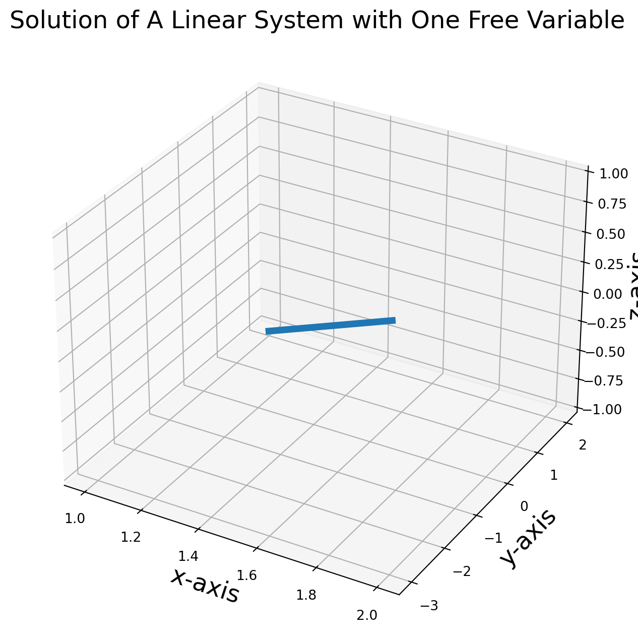
Two Free Variables Case
Now consider the linear system: \[ \left[ \begin{matrix} 1 & -3 & -2\\ 0 &0 & 0 \\ 0& 0 & 0 \end{matrix} \right] \left[ \begin{matrix} x_1\\ x_2\\ x_3 \end{matrix} \right] = \left[ \begin{matrix} 0\\0\\0 \end{matrix} \right] \] The augmented matrix is \[ \left[ \begin{matrix} 1 & -3 & -2 & 0\\ 0 &0 & 0 & 0\\ 0& 0 & 0 & 0 \end{matrix} \right] \] We have two free variables \[ \begin{align} x_1 &= 3x_2+2x_3\\ x_2 &= free\\ x_3 &= free \end{align} \] Rewrite the solution
\[
\left[
\begin{matrix}
x_1\\
x_2\\
x_3
\end{matrix}
\right]
=
\left[
\begin{matrix}
3x_2+2x_3\\
x_2\\
x_3
\end{matrix}
\right]
=
\left[\begin{array}{c}
3 x_{2} \\
x_{2} \\
0
\end{array}\right]+\left[\begin{array}{c}
2 x_{3} \\
0 \\
x_{3}
\end{array}\right]=
x_{2}\left[\begin{array}{l}
3 \\
1 \\
0
\end{array}\right]+x_{3}\left[\begin{array}{l}
2 \\
0 \\
1
\end{array}\right]
\] The solution is a plain spanned by two vectors \((3, 1, 0)^T\) and \((2, 0, 1)^T\). Let’s draw the plane and spanning vectors. We also plot another vector \(v = (2,2,1)\) which is not a linear combination of \((3, 1, 0)^T\) and \((2, 0, 1)^T\). As you pan around the view angle (in JupyterLab use %matplotlib widge), it is apparent that \(v\) is not in the same plane of basis vectors.
fig = plt.figure(figsize=(8, 8))
ax = fig.add_subplot(projection="3d")

x2 = np.linspace(-2, 2, 10)
x3 = np.linspace(-2, 2, 10)
X2, X3 = np.meshgrid(x2, x3)
X1 = 3 * X2 + 2 * X3
ax.plot_wireframe(X1, X2, X3, linewidth=1.5, color="k", alpha=0.6)

vec = np.array(
    [
        [[0, 0, 0, 3, 1, 0]],
        [[0, 0, 0, 2, 0, 1]],
        [[0, 0, 0, 5, 1, 1]],
        [[0, 0, 0, 2, 2, 1]],
    ]
)
colors = ["r", "b", "g", "purple"]
for i in range(vec.shape[0]):
    X, Y, Z, U, V, W = zip(*vec[i, :, :])
    ax.quiver(
        X,
        Y,
        Z,
        U,
        V,
        W,
        length=1,
        normalize=False,
        color=colors[i],
        arrow_length_ratio=0.08,
        pivot="tail",
        linestyles="solid",
        linewidths=3,
        alpha=0.6,
    )

################################Dashed Line################################

point12 = np.array([[2, 0, 1], [5, 1, 1]])
ax.plot(
    point12[:, 0], point12[:, 1], point12[:, 2], lw=3, ls="--", color="black", alpha=0.5
)

point34 = np.array([[3, 1, 0], [5, 1, 1]])
ax.plot(
    point34[:, 0], point34[:, 1], point34[:, 2], lw=3, ls="--", color="black", alpha=0.5
)

#################################Texts#######################################
ax.text(x=3, y=1, z=0, s="$(3, 1, 0)$", color="red", size=16)
ax.text(x=2, y=0, z=1, s="$(2, 0, 1)$", color="blue", size=16)
ax.text(x=5, y=1, z=1, s="$(5, 1, 1)$", color="green", size=16)
ax.text(x=2, y=2, z=1, s="$v$", color="purple", size=16)

ax.set_xlabel("x-axis", size=18)
ax.set_ylabel("y-axis", size=18)
ax.set_zlabel("z-axis", size=18)

ax.view_init(elev=-29, azim=130)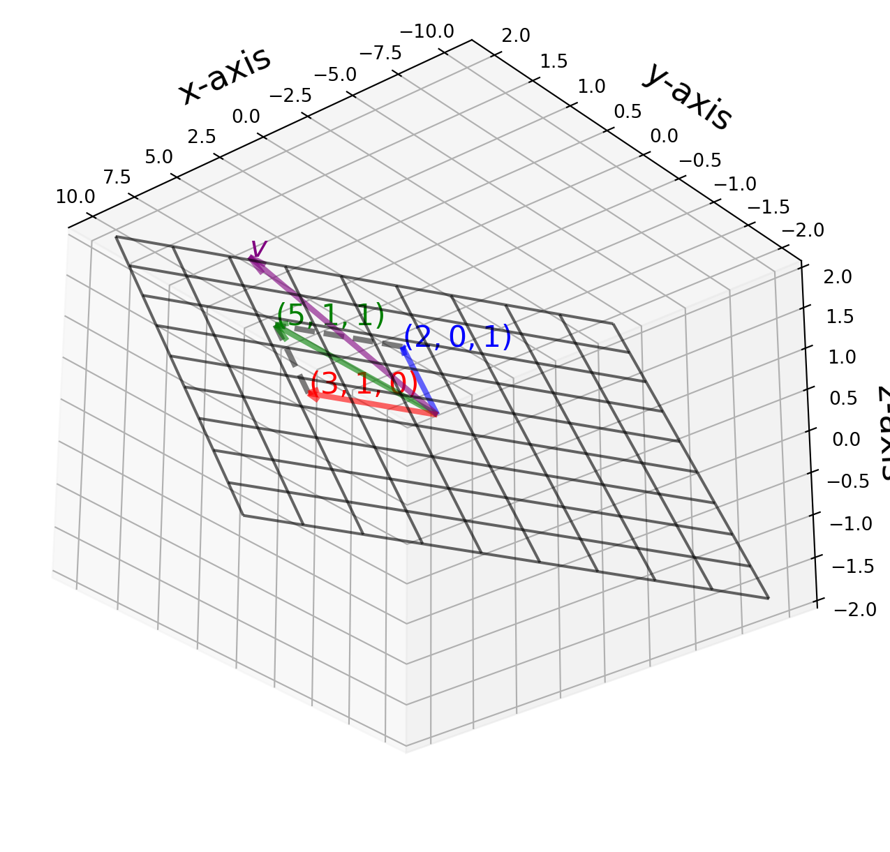
Linear Combination of Polynomial
In a more general sense, a function or a polynomial can also be a linear combination of other functions or polynomials.
Now consider a polynomial \(p(x)=4 x^{3}+5 x^{2}-2 x+7\), determine if it is a linear combination of three polynomials below: \[ p_{1}(x)=x^{3}+2 x^{2}-x+1\\ p_{2}(x)=2 x^{3}+x^{2}-x+1\\ p_{3}(x)=x^{3}-x^{2}-x-4 \]
which means that we need to figure out if the equation below holds
\[ c_{1}\left(x^{3}+2 x^{2}-x+1\right)+c_{2}\left(2 x^{3}+x^{2}-x+1\right)+c_{3}\left(x^{3}-x^{2}-x-4\right)=4 x^{3}+5 x^{2}-2 x+7 \]
Rearrange and collect terms \[ \left(c_{1}+2 c_{2}+c_{3}\right) x^{3}+\left(2 c_{1}+c_{2}-c_{3}\right) x^{2}+\left(-c_{1}-c_{2}-c_{3}\right) x+\left(c_{1}+c_{2}-4 c_{3}\right)=4 x^{3}+5 x^{2}-2 x+7 \]
Equate the coefficients and extract the augmented matrix \[ \begin{aligned} &c_{1}+2 c_{2}+c_{3}=4\\ &2 c_{1}+c_{2}-c_{3}=5\\ &-c_{1}-c_{2}-c_{3}=-2\\ &c_{1}+c_{2}-4 c_{3}=7\\ &\left[\begin{array}{cccc} 1 & 2 & 1 & 3 \\ 2 & 1 & -1 & 5 \\ -1 & -1 & -1 & -2 \\ 1 & 1 & -4 & 7 \end{array}\right] \end{aligned} \]
Before solving, we notice that the system has 4 equations, but 3 unknowns, this case is called over-determined.
A = sy.Matrix([[1, 2, 1, 4], [2, 1, -1, 5], [-1, -1, -1, -2], [1, 1, -4, 7]])
A.rref()
\(\displaystyle \left( \left[\begin{matrix}1 & 0 & 0 & 1\\0 & 1 & 0 & 2\\0 & 0 & 1 & -1\\0 & 0 & 0 & 0\end{matrix}\right], \ \left( 0, \ 1, \ 2\right)\right)\)
We get the answer \((c_1, c_2, c_3)^T = (1, 2, -1)^T\), plug in back to equation \[ \left(x^{3}+2 x^{2}-x+1\right)+2\left(2 x^{3}+x^{2}-x+1\right)-\left(x^{3}-x^{2}-x-4\right)=4 x^{3}+5 x^{2}-2 x+7 \] Indeed we have just established a linear combination between these polynomials.